Uncertainty in Deep Learning
Nowadays, deep learning has found its applications in almost every aspect of our life: from personal assistants such as Siri to various medical applications (e.g. cancer prediction) and autonomous cars. We continue to delegate more and more important tasks to machines and hope they will perform well, e.g:
- Algorithmic trading and Portfolio management
- Human resources and recruiting
- Hospitals and medicine
- Media and e-commerce
- Online and telephone customer service
and many more. Therefore now it’s crucial for such systems not only to make fast and precise prediction, but to provide a measure of its confidence in this prediction.
Example listed above brings us to the area of Uncertainty Estimation in deep learning. In this post we’ll discuss different approaches to this task (including fancy Bayesian models) and learn number of applications of this technology.
Problem statement
Let’s start with formal definition of problem: assume that training dataset consists of i.i.d. samples \(D = \{x_i, y_i\}_{i=1}^N\), where \(x \in \mathbb{R}^n\) and \(y \in \{1, ..., K\}\) are features and categorical labels respectively (for classification task; for regression we have \(y \in \mathbb{R}\)). Our goal is to model probabilistic distrubution \(p_{data}(y \mid x)\) with our predictive distribution \(p_{\theta}(y \mid x)\), where \(\theta\) is parameters of our Neural Network.
Different types of uncertainty
In bayesian framework uncertainty comes from several sources:
- data (aleatoric) uncertainty
- model (epistemic) uncertainty
Aleatoric uncertainty
In our classification example data uncertainty could be expressed with \(p_{data}(y \mid x)\) distribution - this type of uncertainty is irreducible and arises from label noise, class overlaps and other types of noises.
Let’s look at the following example, assume that we’re trying to solve task of cat/dog classification. But then we get this picture in our training dataset:
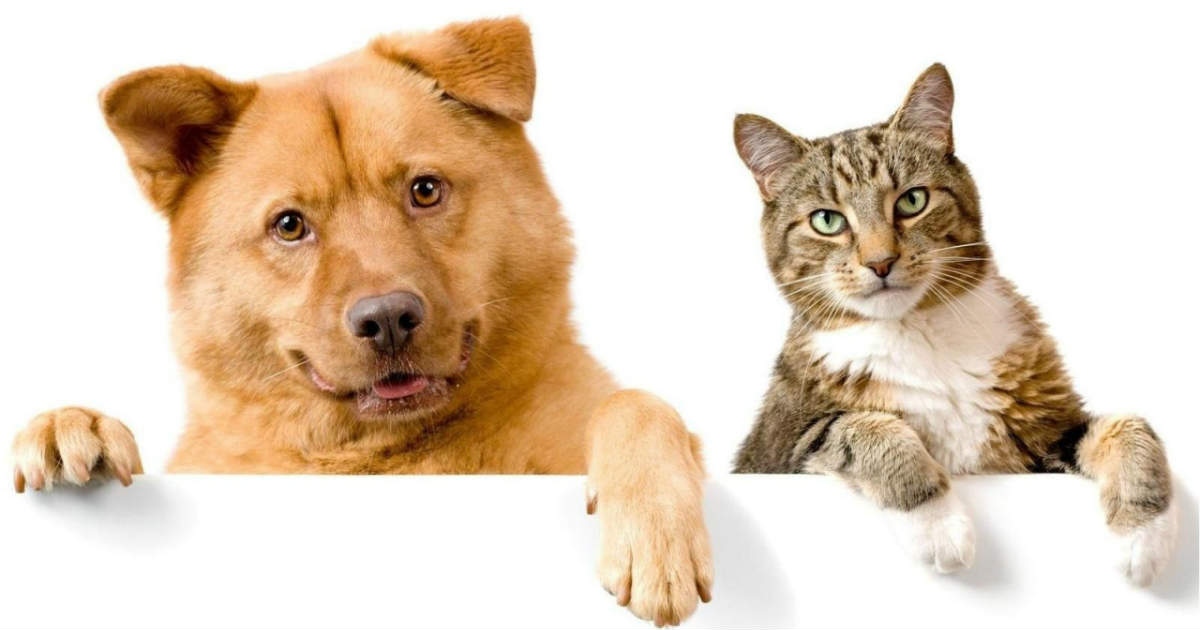
It’s rather hard to say if this picture is “cat” or “dog” class, therefore \(p_{data}(y="dog" \mid x) = 0.5\) and \(p_{data}(y="cat" \mid x) = 0.5\). In this case, it’s impossible to predict certain class for this image and our model should be very uncertain about its predictions. Conversely, for the following image:

the answer is exact - “cat”, thus data uncertainty is low for this particular sample and it’s easy to predict the right label.
In some sence data uncertainty can be considered as “know-unknow”, since our model aware of data complexity and can confidentely state whether it’s hard to classify given sample or not.
Epistemic uncertainty
To understand this type of uncertainty, we should recall some basics about Bayesian inference and its application to uncertainty estimation.
If we want to predict label and estimate uncertainty for new unseen image, then we can formalize this desire in the manner of probabilistic distribution: \(p_{\theta}(y \mid x^{*}, D)\), where \(D\) is training dataset, \(x^{*}\) is unseen input and \(y\) is predicted label. By law of total probability this value can be derived as:
\[p_{\theta}(y \mid x^{*}, D) = \int p(y \mid x^{*}, \theta) \cdot p(\theta \mid D) d\theta \label{eq1}\tag{1}\]and model uncertainty there is expressed via distribution \(p(\theta \mid D)\). Unfortunately, but distribution \(p(\theta \mid D)\) is intractable via Bayes rule:
\[p(\theta \mid D) = \frac{P(D \mid \theta) \cdot P(\theta)}{P(D)}\]since we can’t estimate denominator \(P(D)\), whereas both other factors \(P(D \mid \theta)\) and \(P(\theta)\) are tractable: \(P(\theta)\) is our prior on network weights, often it’s \(\mathcal{N}(0, \sigma \cdot I)\) and \(P(D \mid \theta)\) is part of our probabilistic model (e.g. for regression with MSE loss \(P(y \mid x, \theta) = \mathcal{N} (\mu, \sigma)\)).
Because of this intractability it’s necessary to use either an explicit or implicit variational approximation \(q(\theta)\):
\[q(\theta) \approx p(\theta \mid D)\]However, in models with huge number of parameters (e.g. neural networks) integral in \((\ref{eq1})\) is intractable, therefore MC sampling is commonly used to compute approximation. Ok, now we know, what we need to compute, but how? One of the most popular methods to acquire \(q(\theta)\) is variational inference.
Variational inference
So far we defined variational distribution \(q_\omega(\theta)\), where \(\omega\) are parameters of this distribution. In general, \(q_\omega(\theta)\) should have simple structure and be easy to evaluate. We would like our approximating distribution to be as close as possible to the posterior distribution \(p(\theta \mid D)\), thus we’re going to minimise the Kullback-Leibler (KL) divergence between this distributions:
\[KL(q_{\omega}(\theta) \| p(\theta | D) = \int q_{\omega}(\theta) \log{\frac{q_{\omega}(\theta)}{p(\theta | D)}} d\theta \underset{\omega}{\rightarrow} min \label{eq2}\tag{2}\]Denote solution of this task as \(q_{\omega}^{\ast}(\theta)\). Since distrubutiond \(q_{\omega}^{\ast}(\theta)\) and \(p(\theta \mid D)\) are close in sense of KL divergence, then we could use following approximation:
\[p(y^{\ast} | x^{\ast}, D) \approx \int p(y^{\ast} | x^{\ast}, \theta) \cdot q_{\omega}^{\ast}(\theta) d\theta =: q_{\omega}^{\ast}(y^{\ast}|x^{\ast})\]After some manipulations with definition of KL divergence in \((\ref{eq2})\) we could get
\[KL(q_{\omega}(\theta) \| p(\theta | D) = \int q_{\omega}(\theta)\log{q_{\omega}(\theta)} - \int q_{\omega}(\theta) \log{p(\theta | D)} =\] \[= \int q_{\omega}(\theta)\log{q_{\omega}(\theta)} - \int q_{\omega}(\theta) \log{p(\theta \mid X, Y)} = \int q_{\omega}(\theta)\log{q_{\omega}(\theta)} - \phantom{}\] \[- \int q_{\omega}(\theta) \log{\frac{p(Y \mid \theta, X) \cdot p(\theta)}{p(Y | X)}} = KL(q_{\omega}(\theta) \| p(\theta)) - \int q_{\omega}(\theta) \log{p(Y \mid X, \theta)} + \phantom{}\] \[+ \log{p(Y | X)}\]Since \(KL(q_{\omega}(\theta) \| p(\theta \mid D) \ge 0\), then we can rewrite our minimisation task as maximisation of the evidence lower bound (ELBO) w.r.t. the variational parameters \(\omega\):
\[\mathcal{L}_{VI}(\omega) = \int q_{\omega}(\theta) \log{p(Y \mid X, \theta)} - KL(q_{\omega}(\theta) \| p(\theta)) \le \log{p(Y \mid X)}\]After optimization of VI loss function, we get approximative distribution \(q_{\omega}^{\ast}(\theta) \approx p(\theta \mid D)\) and now we’re able to do inference in our model. In some sense, inference procedure here is rather straight forward: we just sample weights from \(q_{\omega}^{\ast}(\theta)\) and compute forward pass through the network:
\[q_{\omega}^{\ast}(y^{\ast}|x^{\ast}) := \frac{1}{T}\sum_{t=1}^T p(y^{\ast} | x^{\ast}, \theta_t) \underset{T \rightarrow +\infty}{\longrightarrow} \int p(y^{\ast}| x^{\ast}, \theta) \cdot q_{\omega}(\theta) d\theta \approx p(y^{\ast} | x^{\ast}, X, Y)\] \[\theta_t \sim q_{\omega}(\theta)\]Don’t confuse model prediction and uncertainty
In case of classification it seems rather logical to treat predicted probabilities as a measure of model uncertainty. For example, if we’re trying to solve classification task on MNIST, but we use only 0-8 samples during training and never show 9 to our model. Then we assume that for 0-8 samples model will give confident predictions.
Consider some examples: on the following image we have “2” and as expected our network returns confident prediction.

In case of “7” example things become more complicated, since now it’s harder to identify the right class for sample (whether it’s 7 or 1). This is an exact example of aleatoric (data) uncertainty, where troubles come from natural complexity of data.

Now lets feed network with “9” class sample. Model has never seen this kind of data, therefore it should be very uncertain about its prediction. We could expect predictive distribution to be flat and with high entropy, but in the real world our model could return everything.

For neural network models it’s common feature to produce overconfident predictions [1], thus even in case of “9” sample model could return confident prediction with maximum probability e.g. in “4”. That the reason why we should not use outputs of model as measure of uncertainty.
Methods
Gaussian Processes
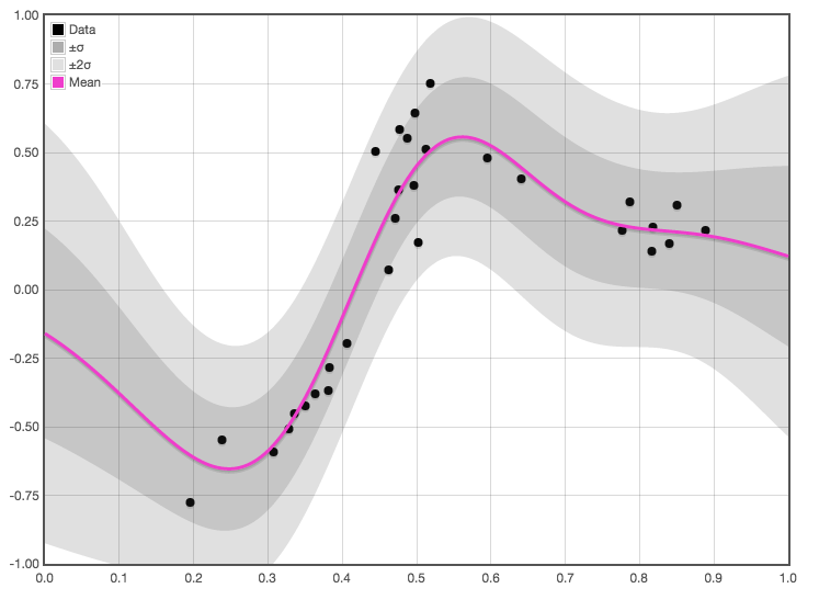
The Gaussian process is a powerful tool in statistics that allows to model distributions over functions. This model offers a range of useful properties such as natural uncertainty estimates over function values and robustness ot over-fitting.
Given a training dataset of pairs \(x \in \mathbb{R}^k\), \(y \in \mathbb{R}^n\) we want to estimate the most probable function \(f(x) = y\) that could generate these observations. For that we define random gaussian process, which is basicly some kind of random function completely defined by mean function \(\mu\) and covariance function \(k\):
\[\mu(x): \mathbb{R}^k \rightarrow \mathbb{R}\] \[k(x, y): \mathbb{R}^k \times \mathbb{R}^k \rightarrow \mathbb{R}_{+}\]We use these functions as a prior for Gaussian Process and training data to calculate probabilities conditioned on this data. In this pipeline, we can calculate probabilistic distribution over outputs in every input point we’re interested, thus results in natural representation of uncertainty of prediction in the given point.
Distributional Parameter Estimation
That’s one of the most straight-forward approach of listed there. Often machine learning model are based on some probabilistic model of data. For example, if we presume that distribution of output \(y\) conditioned on inputs \(x\) and model weighs \(\theta\) has Gaussian structure:
\[p(y | x, \theta) = \mathcal{N}(\mu_{\theta}(x), \sigma)\](where \(\sigma\) is fixed for homoscedastic case), then optimization of log-likelyhood will result in minimization of MSE loss.
\[\mathcal{L}_{MSE} = \frac{1}{N} \sum_i (y_i - f_{\theta}(x_i))^2\]Considering \(\sigma\) as trainable parameter make it possible to treat this quantity as estimation of uncertainty (that depend on input). In this setup loss function will be
\[\mathcal{L} = \frac{1}{N} \sum_i \log{\sigma(x_i)} + \frac{(f_{\theta}(x_i) - y_i)^2}{\sigma^2(x_i)}\]It’s easy to mention, that if model predicts \(f_{\theta}(x_i)\) with high error, than second term in loss could be reduced with larger \(\sigma(x_i)\). First term of loss force \(\sigma(x_i)\) not to be too large, since large values of \(\sigma(x_i)\) would nullify second term.
Idea of likelihood optimization could be applied to any other distribution in which we can control standard deviation. In general, this approach helps us to estimate aleatoric uncertainty and work best when we have a huge amount of training data.
MC Dropout
Dropout is very popular technique used in order to avoid model over-fitting. The idea of Dropout layer is rather simple: during training of our network we’re going to “drop out” random activation maps of previous layer multiplying them by zero, so at every step of training (on every new batch) inference is made on different subsets of weights.


This procedure can be considered as a kind of regularization for network, since it deals with problem of “neurons co-adaptation” [2], when behavior of particular neuron become highly correlated with behavior of another one.
During test time we need to scale down weight, which were dropped out during train time with \(p\) - probability to retain this particular neuron. In general, Dropout shows good results, but sometimes it could cause slight decrease in accuracy of model (in comparison with model without dropout).
MC Dropout is a logical continuation of the Dropout applied to uncertainty estimation, since it was proved in [3] that several stochastic forward passes of network with Dropout can be considered as Appoximate Bayesian Inference. In the nutshell, MC Dropout works as follows:
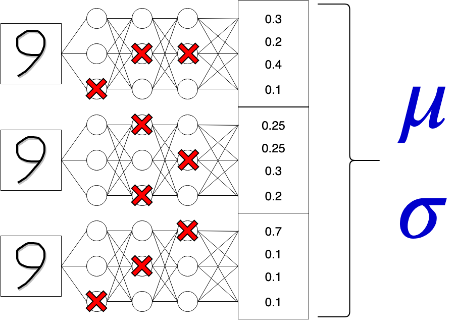
After training of network with Dropout weights of model shouldn’t be scaled and fixed, but instead several forward passes with turned on Dropout are made, what injects randomness in our prediction and allows to model complex distribution over outputs.
After we acquire batch of outputs \(\{y_i\}_{i=1}^T\) from the same input \(x_i\), then we could estimate first two moments of output distribution and consider mean as prediction of model and standart deviation as uncertainty measure. We expect that implicit posterior distribution \(q_{\omega}(\theta)\) over model weights induced by activated Dropout layers will reflect our belief, that model should have larger uncertainty on unknown data and lower uncertainty on training data.
Despite the fact this approach seems promising, often it shows worse results in sense of accuracy than simple ensembling approach, which is discussed in the next section.
Deep Ensembles
The idea of ensembling is rather simple, but in general it shows good results on variety of tasks and often outperforms other approaches of uncertainty estimation.
Instead of training only one model for our task we’re going to train \(K\) (an ensemble) of them. Since we want this models to be uncorrelted, then we need to use random initialization and stochastic training procedures (e.g. SGD) to achieve that. All this training procedures could be performed in parallel since they are independent.
We expect that on training data all of ensemble members perform similarly, but on unseen data we should face large variation in predictions. During inference we calculate mean prediction of our ensemble and some kind of uncertainty, which is based on ensemble prediction variance. For example, for regression task we have:
\[\mu_{\ast}(x) = \frac{1}{M} \sum_m \mu_{\theta_m}(x)\] \[\sigma_{\ast}^{2}(x) = \frac{1}{M} \sum_m (\sigma^2_{\theta_m}(x) + \mu^2_{\theta_m})) - \mu^2_{\ast}(x)\]Moreover, in [4] authors applied Adversarial Training (training on adversarial examples [5]) technique and have shown that AT improves quality of predicted uncertainty on bunch on common benchmarks.
Measures of Neural Network Uncertainty
Entropy
Entropy is common quantity used to estimate rate of uniformity of considered distribution and mathematical formula for this quantity looks like:
\[Entropy = -\sum_i p_i \log{p_i}\]Just for an example letэs look at simple case, when we have Bernulli distribution with parameter \(p\). In this setup our Entropy has following form:
\[Entropy = -(1 - p) \log{(1 - p)} - p\log{p}\]Plot of this function is depicted below.
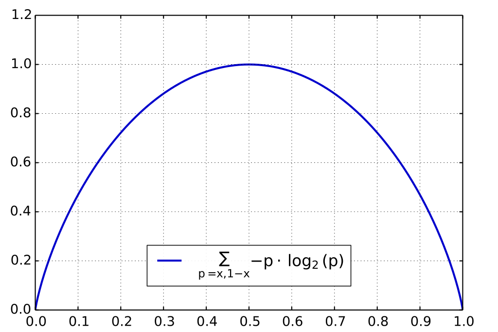
As we can see from this graph entropy is maximazed when \(p = 0.5\), thus when distribution is uniform. Otherwise, when \(p=0\) or \(p=1\) entropy is minimized, what corresponds to degenerate distributions.
This qualities of entropy apply to cases of large dimension distributions, thus we can use this metric as measure of “uniformity” of any distribution. Therefore, entropy turn out to be good data uncertainty measure, when we apply it to in-distribution samples (samples similar to training data).
Hovewer, as it was discussed above, when our model deals with out-of-distribution samples (samples dissimilar to training data) then this approach will fail, since on this type of inputs model could return wrong answers with high confidence (so that’s crucial to manage aleatoric and epistemic uncertainties decomposition).
Mutual information
Mutual information is another quantity widely used in area of Information Theory and in the nutshell mutual information of two random variables is a measure of the mutual dependence between these two variables. General definition of this quantity for two random variables \(X, Y\) is
\[I(X, Y) = D_{KL}(P_{(X, Y)} \| P_{X} \otimes P_{Y})\]but for our purpose it’s much more convenient to use following formula:
\[I(X, Y) = -H(Y|X) + H(Y) = \underset{x \in X}{\sum} P_{X}(x) H(Y|X=x) - \underset{y \in Y}{\sum}P_{Y}(y) \log P_{Y}(y)\]Imagine that we’re working in Variational Inference setup and somehow we’ve learned posterior over model weights \(q_{\omega}(\theta)\) (rather implicitly or explicitly). Therefore now we’re able to sample weights from this distribution and run our model forward pass:
\[\Theta = \{\theta_t\}_{t=1}^T, \theta_t \sim q_{\omega}(\theta)\] \[Y = \{f_{\theta_t}(x)\}_{t=1}^T, \theta_t \in \Theta\](notice, that now we’re working with one particular input \(x\) and consider outputs \(y\) and \(\theta\) as random variables).
Since model weights are variables, then we could measure Mutual Information between output and weights. We assume, that if our outputs have little dependency on model weights, than our model is certain about made predictions.
Missclassification task
As far we’ve already derived some metrics to quantify model uncertainty, then now we need to come up with the idea where we’re going to apply this quantities. First and the most straight forward task for evaluation in this case is missclassification task.
This task is evaluated in several stages:
- train our model on training data
- evaluate model predictions on testing data
- calculate missclassification labels
Interpretation of this labels is 1’s are missclassified samples and 0’s are samples classified properly. After this manipulations we could use uncertainties estimations for every sample as class scores and feed them with \(Y_{miss}\) directly into AUC metrics.
In this pipeline our hope is that model is going to be more uncertain on missclassified samples and more certain on properly classified samples.
Out-of-distribution task
Out-of-distribution task is very similar to previous missclassification task despite several modifications. Now along with our training dataset with need to add one another dataset from another domain (e.g. we could take MNIST and Fashion MNIST datasets), that’s why it called out-of-distribution dataset.
After training, we’re going to prescribe 0’s to images from test part of training dataset and 1’s to out-of-distribution samples from second dataset. In the same manner as for missclassification task we could measure AUC metrics based on uncertainties and earlier prescribed classes.
For this task we assume that model is going to be more uncertain on samples from another domain, but for in-distribution samples uncertainty would be rather small.
Conclusion
Uncertainty Estimation task is still very important and hot problem, which is not fully solved at the moment. In the same time a lot of different areas could benefit from advances in this area: such as self-driving cars, robotics, medical application and etc.
Despite powerful theoretical grounding of MC Dropout and Bayesian Method used for this task often they produce unsatisfying uncertainty estimations for real world applications. In the same time, such common approach as ensembling has huge overhead in sense of computation time and resources (and sometimes it shows unsatisfying results too), therefore it could be impossible to use it on embedded devices or for low latency applications.
References
[1] Guo, Chuan and Pleiss, Geoff and Sun, Yu and Weinberger, Kilian Q., On Calibration of Modern Neural Networks
[2] Srivastava, Nitish and Hinton, Geoffrey and Krizhevsky, Alex and Sutskever, Ilya and Salakhutdinov, Ruslan, Dropout: A Simple Way to Prevent Neural Networks from Overfitting
[3] Gal, Yarin and Ghahramani, Zoubin, Dropout As a Bayesian Approximation: Representing Model Uncertainty in Deep Learning
[4] Lakshminarayanan, Balaji and Pritzel, Alexander and Blundell, Charles, Simple and Scalable Predictive Uncertainty Estimation Using Deep Ensembles
[5] Ian Goodfellow and Jonathon Shlens and Christian Szegedy, Explaining and Harnessing Adversarial Examples