Uncertainty at ICLR 2020
ICLR это одна из самых больших и влиятельных конференций по исскуственному интеллекту и дип лернингу в мире, на которой публикуются тысячи статей по тематике каждый год.
In particular, ICLR 2020 brought a lot of valuable insights about uncertainty of modern deep learning models and in this post I would like to describe shortly the most interesting papers which were presented during the conference on this topic.
Content:
- Hypermodels for Exploration
- Bayesian Meta Sampling for Fast Uncertainty Adaptation
- Uncertainty-guided Continual Learning with Bayesian Neural Networks
Hypermodels for Exploration
Hypermodels (or originally “HyperNetworks”) это подход который призван сделать обучение ансамблей нейросетей простым и дешевым: как известно затраты на обучение ансабмлей растут линейно с количеством моделей в них и для некоторых приложений такая динамика совершенно непозволительна.
Авторы оригинальной статьи подошли к этой проблеме сдедующим образом: вместо независимого параллельного обучения нескольких моделей \(\{m_{i} \mid i=\overline{1, n}\}\) можно выучить одну (мета-)модель \(M_{meta} : i \rightarrow m_{i}\), которая будет принимать индекс как вход и на выходе предсказывать другую модель (ее веса). Таким образом единовременно можно будет хранить только веса мета-модели, а сами модели генерировать налету. В более сложных вариантах HyperNetwork может приниматься \(i \in \mathbb{R}\) порождая таким образом неприрывный спектр моделей.
Ансамбли нейросетей являются одним и самых популярных методов для оценики неопределенности моделей: все что нужно сделать это прогнать обучение несколько раз, собрать разные чекпойнты и использовать вариативность их предсказаний как непределенность. Так как HyperNetworks предназначенны как раз для того, чтобы аппроксимировать ансабли, то в статье Hypermodels for Exploration авторы рассмативают вопрос насколько хорошо HyperNetworks могут оценивать неопределенность и использовать ее для более эффективного обучения RL агентов через exploration / exploitation trade-off (например, через Thompson Sampling).
На изображении ниже мы можем увидеть сравнение инференса в обычной и в Hypermodels моделях. Так как авторы работают в RL сетапе, то на вход модели получают текущий вектор состояния среды \(X_t\) и обе модели пытаются предсказать сдедующее действие \(Y_{t+1}\). Главным отличием в пайплайнах является то, что Hypermodels модель сначала семплирует индекс \(z \sim p_{z}\) и только после предсказания весов модели \(\theta = g_{\nu}(z)\) мы получаем конечные предсказания \(Y_{t+1}\).

Тем не менее, все еще главным остается вопрос о том, как производить обучение такой модели? Обычный бекпроп, который так хорошо работает для стандартных модей, не сработает, так как в этом случае мета-модель может выучить игнорировать входной вектор \(z\) и весь смысл будет потерян. Для этого авторы предлагают перед началом обучения для каждого семпла в обучающем датасет нужно сгенерировать \(a \sim \mathcal{N(0, 1)}\) и рассматривать датасет как тройки \((x, y, a)\). В самом лоссе мы модифицируем стандартный MSE добавив в него слагаемое \(\sigma_{w}a^Tz\) как раз для цели разнообразить поведение различных сгенерированных моделей.

Второй слагаемое в данном лоссе представляет своеобразную регуляризацию на то, что сгенерированные веса модели не должны сильно отклоняться от весов сгенерированных мета-моделью инициализированной изначально.
Since author’s motivation for studying hypermodels stems from their potential role in improving exploration methods therefore they evealuate the idea in RL setting with procedure similar to Thompson Sampling.
В качестве результатов авторы предоставляют эксперименты на задачах бандитов и подтверждают, что в сравнение с таким популярными алгоритмами эксплорейшена как ансамбли и eps-greedy их модель показывает намного более быструю сходимость.

Uncertainty-guided Continual Learning with Bayesian Neural Networks
Задача Continual Learning состоит в том, чтобы позволить модели выучивать зависимости на новых поступивших данных и при этом не забывать старые. Типичным примером для задач Continual Learning являются задачи с постоянно растущими данными, например поток поведения клиентов в мобильном приложении: мы постоянно получаем новые данные от новых пользователей по мере их появления, но при этом не хотим забывать поведение старых пользователей.
Мотивация автором данной статьи состоит в том, что байесовский вывод обладает одним очень приятным свойством – при получении новых данных подель вовсе не требует переобучения, так как по формуле байеса:
\[P(\theta | D_{new}) = \frac{P(D_{new} | \theta) \cdot P(\theta)}{P(D_{new})}\]где \(P(\theta)\) представляется наше априорное представление о весах модели. В случае байесовского вывода мы могли обучить нашу модель на старых данных и получить \(P(\theta \mid D_{old})\), а затем использовать выученное распределение в качестве праера для \(P(\theta)\) в формуле выше.
Держа это в голове авторы предлагают использовать Bayes-by-Backprop подход, который по сути представляется из себя mean-field variational inference, а значит выполняет approximate bayes. In the nutshell, данные метод представляет каждый вес модели \(w\) как два: \(\mu\) - среднее, \(\sigma\) - стандартное отклонение и вводит вариационное распределение \(w \sim \mathcal{N}(\mu, \sigma)\), а обучается такая модель потом через \(ELBO\).
A common strategy to perform continual learning is to reduce forgetting by regularizing furtherchanges in the model representation based on parameters’ importance. In provided method the regularization is performed with the learning rate such that the learning rate of each parameter and hence its gradient update becomes a function of its importance.
Более детально, то авторы предлагают апдейтить non-important веса (веса с маленьким \(\sigma\)) меньше, а с большим - больше, таким образом:
\[\alpha_{\mu} \leftarrow \alpha_{\mu} \cdot \sigma\]Таким образом веса, в которых модель будет уверенна будут слабо изменяться во время обучения, в то время как остальные веса будут получать более высокий learning rate.
Conservative Uncertainty Estimation By Fitting Prior Networks
Prior Networks is a rather new idea, which was applied to uncertainty estimation task recently in several papers (don't confuse it with Prior Networks from [1]). Originaly it was used for improved exploration in reinforcement learning tasks and it has showed promising result on a range of benchmarks. In general, this approach really resembles simple ensembling method, but at the same time it has several substantial drawbacks and advantages comparing with it.
So, how it works? First of all we need to create \(N\) different randomly initialized networks, which won’t be trained ever. This networks are callled Prior Networks and they are a core idea of this approch. Since we are solving some deep learning task, then we have a training dataset \(\{X, y\}\) and second step in this algorithm consists of evaluating every Prior Network \(f\) on training set samples \(\{f_i(X)\}_{i=1}^{N}\). Then this set of evaluated outputs is used to train another set of models \(\{h_i\}_{i=1}^N\) called Predictor Networks:
\[h_i = FIT(h_i, X, f_i(X))\]That’s it, we are trying to make every Predictor Network to match predictions of Prior Networks on training samples. When all that is done, then in order to obtain uncertainty for particular example \(x_{\star}\) we need to run inference on all Prior Networks and Predictor Networks and use differences in their predictions to quantify uncertainty:
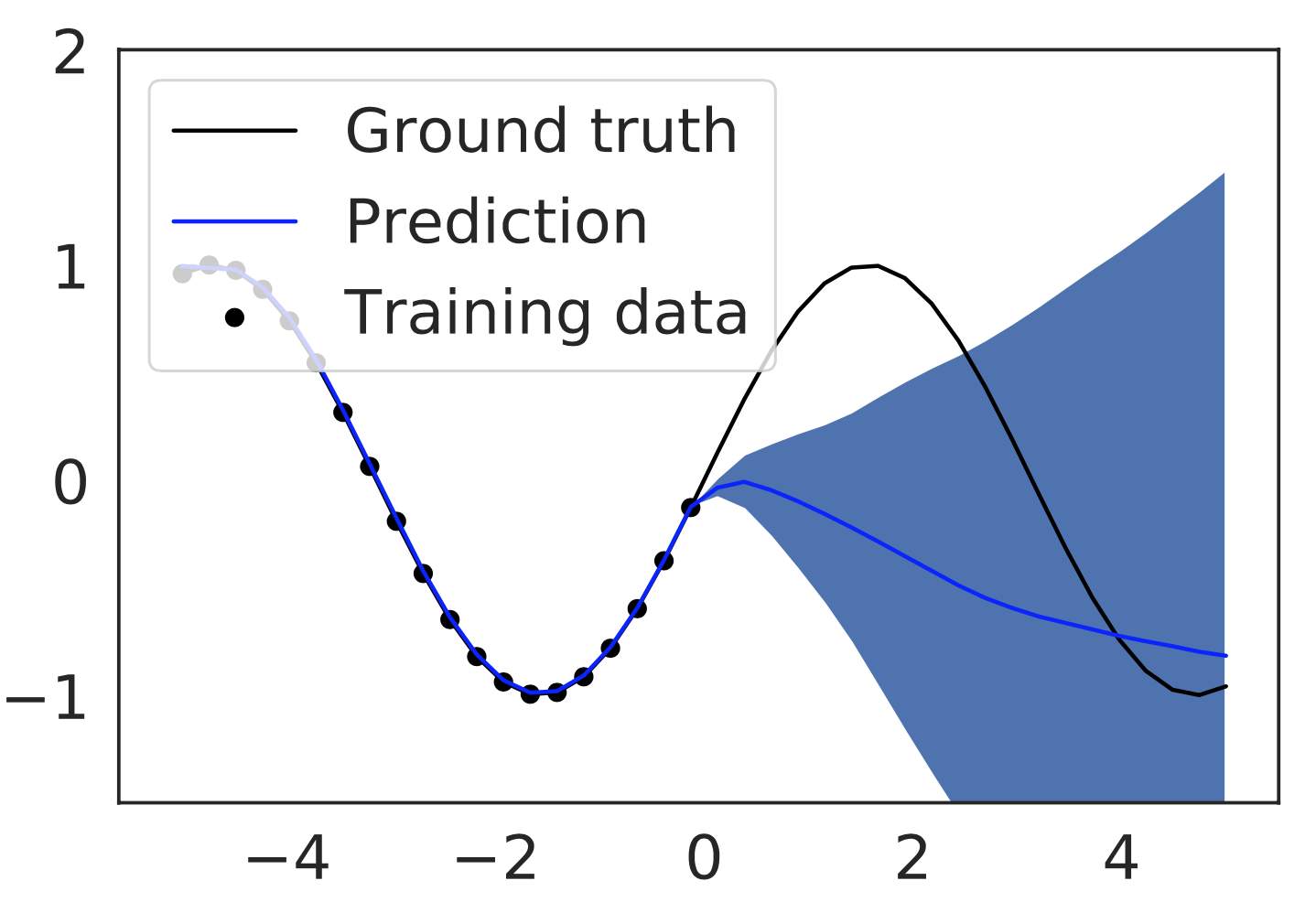
\[\hat{\sigma}_{\mu}^2(x_{\star}) = \frac{1}{N} ||f_{i}(x_{\star}) - h_{i}(x_{\star})||^2\]Here are some examples from original paper:
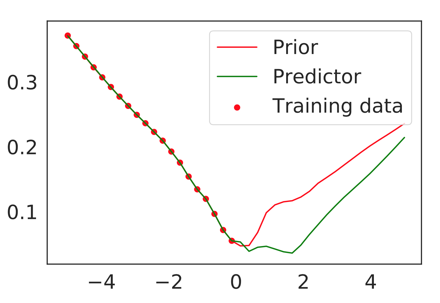
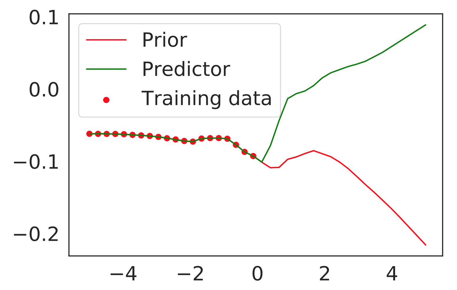
As far as we can see, both Prior and Predictor models show similar predictions on training data, but on out-of-distribution domain their predictions differ significantly.
Eventually, that’s the core idea of this method: as well as for ensembles we believe, that different models would show similar predictions for samples that are close to training data, but in the same time they will behave differently on out-of-distribution samples. In this case, we hope that Prior and Predictor Networks will behave in simillar manner.
Another cool property of this approach is that for mean prediction we train absolutely separate network, which will never interact with Prior/Predictor networks at all. Therefore, if you’ve already trained a model and it performs great, but you would like to get uncertainty in addition, then this approach could be usefull.
Moreover, it’s important to note that authors have provided theoretical justification of their algorithm, which is based on Gaussian Processes formalism. In their proofs they have showed, that with their approach you will never underestimate uncertainty (Conservative property) and with \(\lim_{B, D \rightarrow \infty}\) (\(B\) - number of prior networks, \(D\) - number of training samples) their method will converge to real uncertainties of Gaussian Process posterior (Concentration property).
Unfortunately, but authors didn’t provide extensive experimental support for their method (only image classification tasks), but on them they have demonstrated sustainably good results.
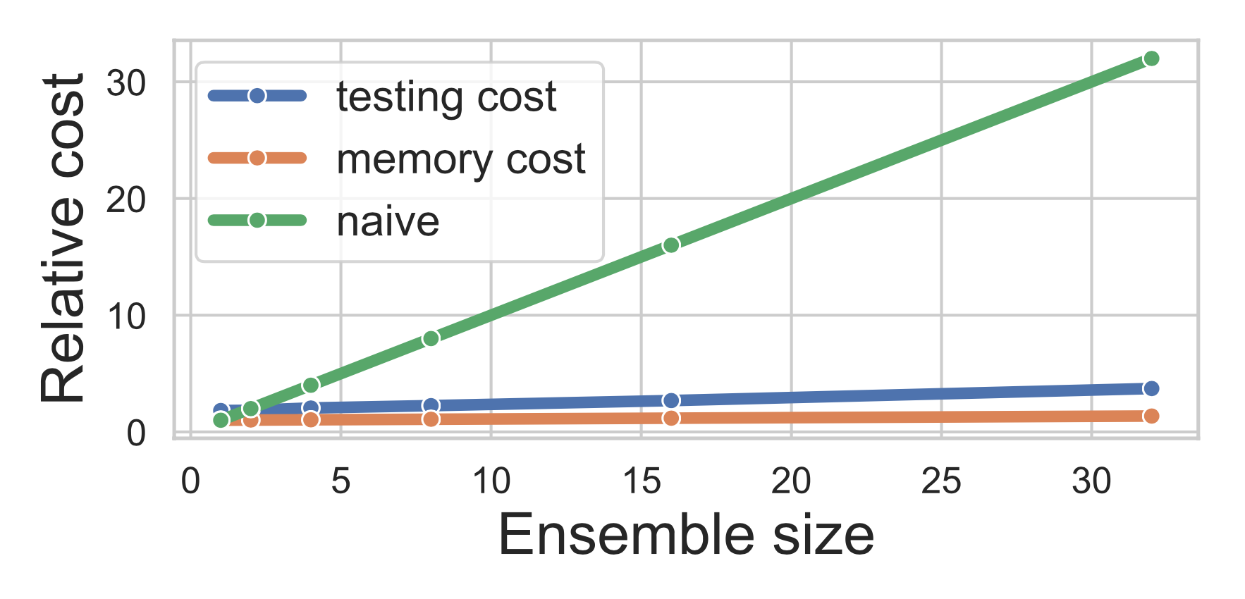
The only strong disadvantage of this approach that make it hard to apply Prior Networks to real world applications is: eventually you need to use \(B\) times more memory to store all this Prior/Predictor networks (or even more, because of Prior Networks) and train \(B\) times more models, but in the same time you will use only one of them for final predictions. From perspective of ensembles, where we use all of trained networks for inference, Prior Networks should suffer from lower accuracy performance.
BatchEnsemble: an Alternative Approach to Efficient Ensemble and Lifelong Learning
One of the most discouraging things about ensembles of Deep Networks is memory and computational overheads. In case of vanilla implementation of Deep Ensembles memory overhead and training time are \(N\) times more comparing with single model costs. In BatchEnsemble paper authors aim to address these computational and memory issues by building efficient ensemling method.
But since Ensembles still tend to outper Variational Bayesian Network [2] in terms of both accuracy and uncertainty metrics, then there are huge desire to develope ensembling-like method, that could both solve memory issues and achieve comparable quality as ensembles.
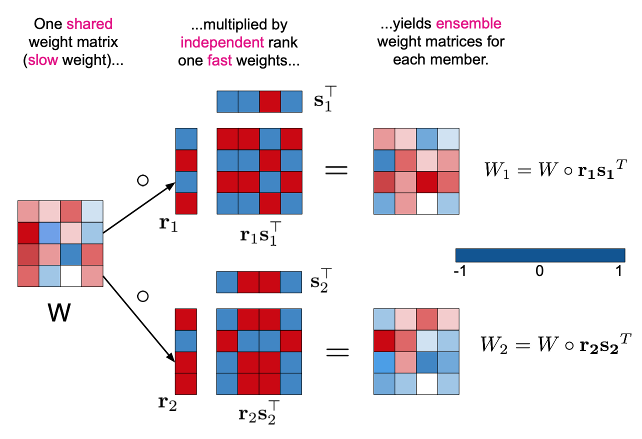
With this thought in mind authors introduced simple and elegant solution - BatchEnsemble layer. For every model in ensemble and for every BatchEnsemble layer we need to store additional pair on vectors \(p_i\) and \(q_i\). Dimentionality of \(p_i\) is equal to number of channels in inputs activations and dimentionality of \(q_i\) is equal to number of channels in output activations. During forward pass through BatchEnsemble layer inputs activations firstly are multiplied by \(p_i\) (channel-wise), then regular convolution follows, then resulting activations are multiplied by \(q_i\) (channel-wise as well).
As it’s illustrated on Figure 5. such sequence of multiplications could be seen as regular convolution that is modified for every distinct model in “ensemble”. Because of the fact that weights of every separate model are unique, then in this way model tries to mimic vanilla ensembles behaviour.
Extensive experiments on conventional image classification, machine translation problems and application of BatchEnsembles to Continual Learning task proved abilility of this method to produce high quality uncertainty estimations and good model calibration without huge computational overhead assosiated with vanilla ensembles approach.
Pitfalls of In-Domain Uncertainty Estimation and Ensembling in Deep Learning
Ensemble Distribution Distillation
AugMix: A Simple Data Processing Method to Improve Robustness and Uncertainty
References
[1] Andrey Malinin, Mark Gales, Predictive Uncertainty Estimation via Prior Networks [arxiv]
[2] Fredrik K. Gustafsson, Martin Danelljan, Thomas B. Schön, Evaluating Scalable Bayesian Deep Learning Methods for Robust Computer Vision [arxiv]